Exploring Major Cities Health Indicator Data

This notebook focus on analysing big cities health indicator data and plot important indicators and changes in different perespective using python language and other data processing and vusualization tolls such as pandas, seaborn, matlibplot, and soon.

Data Description

Data link: Big Cities Health Data Platform

This dataset illustrates health status of 30 of the nation’s largest and most urban cities as captured with diffirent health indicators. These indicators represent some of the leading causes of morbidity and mortality in the United States and leading priorities of national, state, and local health agencies. Public health data were captured in nine overarching categories: HIV/AIDS, cancer, nutrition/physical activity/obesity, food safety, infectious disease, maternal and child health, tobacco, injury/violence, and behavioral health/substance abuse.

import pandas as pd ## for reading and undestanding data
import matplotlib.pyplot as plt ## for plotting data
import seaborn as sns ## another library to visualize data features
import numpy as np ## for numerical array processing

data=pd.read_csv('BCHI-dataset_2019-03-04.csv')#reading csv data to data object with pandas
data.shape ## shows number of rows and columns

(34492, 15)

data.columns ## shows column names as python tuple

Index(['Indicator Category', 'Indicator', 'Year', 'Sex', 'Race/Ethnicity',
       'Value', 'Place', 'BCHC Requested Methodology', 'Source', 'Methods',
       'Notes', '90% Confidence Level - Low', '90% Confidence Level - High',
       '95% Confidence Level - Low', '95% Confidence Level - High'],
      dtype='object')

The data has 34, 492 data points with 15 features (variables to characterize each data points) depicting ‘Indicator Category’, ‘Indicator’, ‘Year’, ‘Gender’, ‘Race/ Ethnicity’, ‘Value’, ‘Place’, ‘BCHC Requested Methodology’, ‘Source’, ‘Methods’, ‘Notes’‘90% Confidence Level - Low’, ‘90% Confidence Level - High’, ‘95% Confidence Level - Low’, and ‘95% Confidence Level - High’ for each data points.

Lets inspect first 5 records from data.

Variables such as ‘BCHC Requested Methodology’, ‘Source’, ‘Methods’, ‘Notes’, and confidence level are not important for our analysis, because those variables are included to describe data collection methodology, source of the data, and level for rate defined. Lets drop those variables and inspect the rest

varibles_to_drop = ['BCHC Requested Methodology', 'Source', 'Methods', 'Notes','90% Confidence Level - Low', '90% Confidence Level - High',
       '95% Confidence Level - Low', '95% Confidence Level - High'] # taking all features to be droped as python List object
data=data.drop(varibles_to_drop, axis=1)## drops column cells
data.head() ## displays the fisrt 5 records

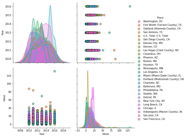
data=data[(data['Indicator Category']=='Behavioral Health/Substance Abuse')]

_=sns.pairplot(data, hue = 'Place', diag_kind = 'kde', plot_kws = {'alpha': 0.6, 's': 80, 'edgecolor': 'k'}, height = 4);

data[(data['Indicator Category']=='HIV/AIDS')].head()

d=data[(data['Indicator Category']=='Behavioral Health/Substance Abuse')]

d[(d['Indicator']=='Percent of High School Students Who Binge Drank')]

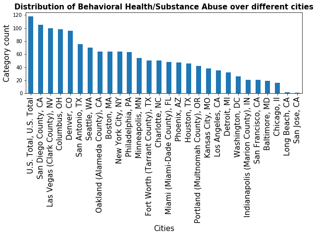
def plot_indicator_per_cities(category,data_count):
    fig, ax = plt.subplots(figsize=(10, 3))
    ax.tick_params(axis='x', labelsize=15)
    ax.tick_params(axis='y', labelsize=10)
    ax.set_xlabel('Cities', fontsize=15)
    ax.set_ylabel('Category count' , fontsize=15)
    ax.set_title('Distribution of {} over different cities'.format(category), fontsize=15, fontweight='bold')
    _=place_count.plot(ax=ax, kind='bar')

from datetime import datetime
dt=str(2010)
dd=datetime.strptime(dt,'%Y')

data_sub=data.copy()
data_substance=data[(data['Indicator Category']=='Behavioral Health/Substance Abuse')]
data_sex=data[(data['Indicator Category']=='Sexually Transmitted Infections')]
data_cancer=data[(data['Indicator Category']=='Cancer')]

## all cancer, lung cancer, breast cancer mortality rate
## yearly brest cancer mortality rate accross all countries
## country wide for selected countries
place_count=data_substance['Place'].value_counts() 
plot_indicator_per_cities('Behavioral Health/Substance Abuse',place_count)

all_cancer=data_cancer[(data_cancer['Indicator']=='All Types of Cancer Mortality Rate (Age-Adjusted; Per 100,000 people)')]
all_cancer=data_cancer[['Year','Value']]
all_cancer = all_cancer.dropna(how='any',axis=0)
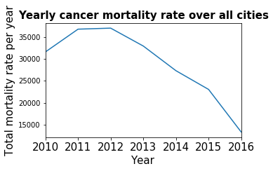
cancer_by_year=all_cancer.groupby('Year')['Value'].sum()
fig, ax = plt.subplots(figsize=(5, 3))
plt.title('Yearly cancer mortality rate over all cities')
plt.ylabel('Total mortality rate per year')
plt.xlabel('Years')
ax.tick_params(axis='x', labelsize=15)
ax.tick_params(axis='y', labelsize=10)
ax.set_xlabel('Years', fontsize=15)
ax.set_ylabel('Total mortality rate per year' , fontsize=15)
ax.set_title('Yearly cancer mortality rate over all cities', fontsize=15, fontweight='bold')
_=cancer_by_year.plot(kind='line')
# plt.show()

# all_cancer=data_cancer[(data_cancer['Indicator']=='Lung Cancer Mortality Rate (Age-Adjusted; Per 100,000 people)') & (data_cancer['Place']=='Boston, MA')]
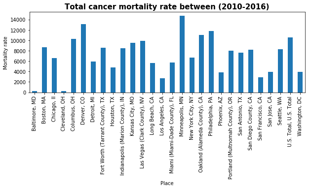
all_cancer=data_cancer[['Place','Value']]
all_cancer = all_cancer.dropna(how='any',axis=0)
cancer_boston=all_cancer.groupby('Place')['Value'].sum()
fig, ax = plt.subplots(figsize=(10, 3))
ax.tick_params(axis='x', labelsize=10)
ax.tick_params(axis='y', labelsize=10)
ax.set_xlabel('Cities', fontsize=10)
ax.set_ylabel('Mortality rate' , fontsize=10)
ax.set_title('Total cancer mortality rate between (2010-2016)', fontsize=15, fontweight='bold')
_=cancer_boston.plot(kind='bar')

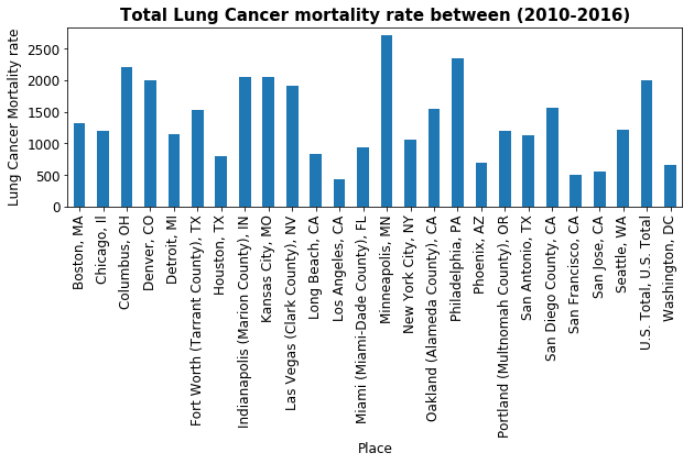
lung_cancer=data_cancer[(data_cancer['Indicator']=='Lung Cancer Mortality Rate (Age-Adjusted; Per 100,000 people)')]
#& (data_cancer['Place']=='Boston, MA')
lung_cancer=lung_cancer[['Place','Value']]
lung_cancer = lung_cancer.dropna(how='any',axis=0)
lung_cancer=lung_cancer.groupby('Place')['Value'].sum()
fig, ax = plt.subplots(figsize=(10, 3))
ax.tick_params(axis='x', labelsize=12)
ax.tick_params(axis='y', labelsize=12)
ax.set_xlabel('Cities', fontsize=12)
ax.set_ylabel('Lung Cancer Mortality rate' , fontsize=12)
ax.set_title('Total Lung Cancer mortality rate between (2010-2016)', fontsize=15, fontweight='bold')
_=lung_cancer.plot(kind='bar')

def plot_indicators(y_feature,x_feature,data_sub):
    sns.set(rc={'figure.figsize':(10,10)})
    ax=sns.plot(y=y_feature,hue=x_feature,data=data_sub)
    for p in ax.patches:
        patch_height = p.get_height()
        if np.isnan(patch_height):
            patch_height = 0
        ax.annotate('{}'.format(int(patch_height)), (p.get_x()+0.01, patch_height+3))
    plt.title("Distribution of {} per {}".format(y_feature,x_feature))
    plt.show()

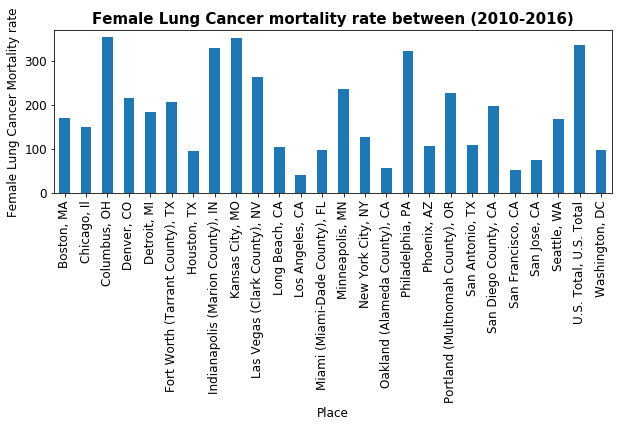
lung_cancer=data_cancer[(data_cancer['Indicator']=='Lung Cancer Mortality Rate (Age-Adjusted; Per 100,000 people)') & (data_cancer['Sex']=='Female')]
#& (data_cancer['Place']=='Boston, MA')
lung_cancer=lung_cancer[['Place','Value']]
lung_cancer = lung_cancer.dropna(how='any',axis=0)
lung_cancer=lung_cancer.groupby('Place')['Value'].sum()
fig, ax = plt.subplots(figsize=(10, 3))
ax.tick_params(axis='x', labelsize=12)
ax.tick_params(axis='y', labelsize=12)
ax.set_xlabel('Cities', fontsize=12)
ax.set_ylabel('Female Lung Cancer Mortality rate' , fontsize=12)
ax.set_title('Female Lung Cancer mortality rate between (2010-2016)', fontsize=15, fontweight='bold')
_=lung_cancer.plot(kind='bar')
# plot_indicators('Value','Place')

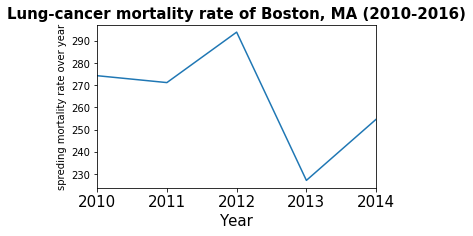
all_cancer=data_cancer[(data_cancer['Indicator']=='Lung Cancer Mortality Rate (Age-Adjusted; Per 100,000 people)') & (data_cancer['Place']=='Boston, MA')]
all_cancer=all_cancer[['Year','Value']]
all_cancer = all_cancer.dropna(how='any',axis=0)
cancer_boston=all_cancer.groupby('Year')['Value'].sum()
fig, ax = plt.subplots(figsize=(5, 3))
ax.tick_params(axis='x', labelsize=15)
ax.tick_params(axis='y', labelsize=10)
ax.set_xlabel('Years', fontsize=15)
ax.set_ylabel('spreding mortality rate over year' , fontsize=10)
ax.set_title('Lung-cancer mortality rate of Boston, MA (2010-2016)', fontsize=15, fontweight='bold')
_=cancer_boston.plot(kind='line')

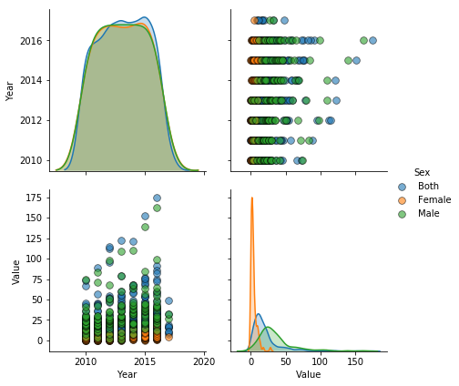
sex_infection=data_sex[(data_sex['Indicator']=='Primary and Secondary Syphilis Rate (Per 100,000 People)')]
# sex_infection=sex_infection[['Place','Year','Value']]
_=sns.pairplot(sex_infection, hue = 'Sex', diag_kind = 'kde', vars=['Year','Value'], plot_kws = {'alpha': 0.6, 's': 60, 'edgecolor': 'k'}, height = 3);

# place_count=data_sex['Place'].value_counts() 
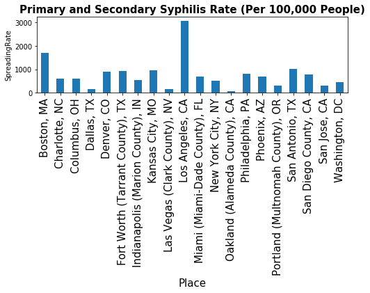
sex_infection=data_sex[(data_sex['Indicator']=='Primary and Secondary Syphilis Rate (Per 100,000 People)')]
sex_infection=sex_infection[['Place','Value']]
sex_infection = sex_infection.dropna(how='any',axis=0)
sex_infection=sex_infection.groupby('Place')['Value'].sum()
print(sex_infection.head())
fig, ax = plt.subplots(figsize=(8, 2))
ax.tick_params(axis='x', labelsize=15)
ax.tick_params(axis='y', labelsize=10)
ax.set_xlabel('Cities', fontsize=15)
ax.set_ylabel('SpreadingRate' , fontsize=10)
ax.set_title('Primary and Secondary Syphilis Rate (Per 100,000 People)', fontsize=15, fontweight='bold')
_=sex_infection.plot(kind='bar')

Place
Boston, MA       1712.6
Charlotte, NC     594.9
Columbus, OH      608.6
Dallas, TX        165.0
Denver, CO        884.0
Name: Value, dtype: float64

# Primary and Secondary Syphilis Rate

data['Indicator Category'].value_counts() 

Chronic Disease                             4854
HIV/AIDS                                    3887
Injury/Violence                             3776
Demographics                                3397
Sexually Transmitted Infections             3348
Infectious Disease                          3082
Cancer                                      2670
Social and Economic Factors                 2573
Maternal and Child Health                   2213
Food Safety                                 1495
Behavioral Health/Substance Abuse           1465
Life Expectancy and Death Rate (Overall)    1424
Environment                                  308
Name: Indicator Category, dtype: int64

data['Methods'].value_counts() 

From this data we can analyse,

1. which countries are commonly attacked by which disease?
2. Disease spreading rate per year for most commonly affected countiries.
3. Which gender or race is commonly attacked?

with aim to give clue for concerned bodies (can be government offical, NGO’s or individuals).